Assignment3

Computer Science - The City College of New York
CSC I6716 - Spring 2015 3D Computer Vision

Assignment 3 Camera Models and Camera Calibration ( Deadline extended to : April 14 Tuesday before class)
(Those marked with * are optional for extra credits)

Note: All the writings must be submitted in hard copies. Please write your **names** and IDs (last four digits) in your submissions.

1   (Camera Models- 20 points) Prove that the vector from the viewpoint of a pinhole camera to the vanishing point (in the image plane) of a set of 3D parallel lines is parallel to the direction of the parallel lines. Please show steps of your proof.

Hint: You can either use geometric reasoning or algebraic calculation.

If you choose to use geometric reasoning, you can use the fact that the projection of a 3D line in space is the intersection of its “interpretation plane” with the image plane. Here the interpretation plane (IP) is a plane passing through the 3D line and the center of projection (viewpoint) of the camera. Also, the interpretation planes of two parallel lines intersect in a line passing through the viewpoint, and the intersection line is parallel to the parallel lines.

If you select to use algebraic calculation, you may use the parametric representation of a 3D line: P = P0 +tV, where P= (X,Y,Z)^T is any point on the line (here ^T denote for transpose),   P0 = (X0,Y0,Z0)^T is a given fixed point on the line, vector V = (a,b,c)^T represents the direction of the line, and t is the scalar parameter that controls the distance (with sign) between P and P0.

2. (Camera Models- 20 points) Show that relation between any image point (xim, yim)^T of a plane (in the form of (x1,x2,x3)^T in projective space ) and its corresponding point (Xw, Yw, Zw)^T on the plane in 3D space can be represented by a 3x3 matrix. You should start from the general form of the camera model (x1,x2,x3)^T = M_intM_ext (Xw, Yw, Zw, 1)^T, where the image center (ox, oy), the focal length f, the scaling factors( sx and sy), the rotation matrix R and the translation vector T are all unknown. Note that in the course slides and the lecture notes, I used a simplified model of the perspective project by assuming ox and oy are known and sx = sy =1, and only discussed the special cases of planes.. So you cannot directly copy those equations I used. Instead you should use the general form of the projective matrix, and the general form of a plane n_x X_w + n_y Y_w + n_z Z_w = d.

3.  (Calibration- 20 points ) Prove the Orthocenter Theorem by geometric arguments: Let T be the triangle on the image plane defined by the three vanishing points of three mutually orthogonal sets of parallel lines in space. Then the image center is the orthocenter of the triangle T (i.e., the common intersection of the three altitudes.
(1)    Basic proof: use the result of Question 1, assuming the aspect ratio of the camera is 1. (10 points)
(2)    If you do not know the focal length of the camera, can you still find the image center (together with the focal length) using the Orthocenter Theorem? Show why or why not. (5 points)
(3)    If you do not know the aspect ratio and the focal length of the camera, can you still find the image center using the Orthocenter Theorem? Show why or why not. (5 points)

4. Calibration Programming Exercises (40 points): Implement the direct parameter calibration method in order to (1) learn how to use SVD to solve systems of linear equations; (2) understand the physical constraints of the camera parameters; and (3) understand important issues related to calibration, such as calibration pattern design, point localization accuracy and robustness of the algorithms. Since calibrating a real camera involves lots of work in calibration pattern design, image processing and error controls as well as solving the equations, we will mainly use simulated data to understand the algorithms. As a by-product we will also learn how to generate 2D images from 3D models using a “virtual” pinhole camera.

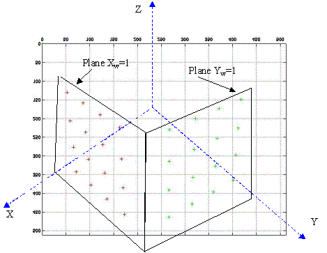
Calibration pattern “design”. Generate data of a “virtual” 3D cube similar to the one shown in Fig. 1 of the lecture notes in camera calibration. For example, you can hypothesize a 1x1x1 m³ cube and pick up coordinates of 3-D points on one corner of each black square in your world coordinate system. Make sure that your data is sufficient for the following calibration procedures. In order to show the correctness of your data, draw your cube (with the control points marked) using Matlab (or whatever tools you are selecting). I have provided a piece of starting code in Matlab for you to use.
“Virtual” camera and images. Design a “virtual” camera with known intrinsic parameters including focal length f, image center (o_x, o_y) and pixel size (s_x, s_y). As an example, you can assume that the focal length is f = 16 mm, the image frame size is 512*512 (pixels) with (o_x,o_y) = (256, 256), and the size of the image sensor inside your camera is 8.8 mm *6.6 mm (so the pixel size is (s_x,s_y) = (8.8/512, 6.6/512) ). Capture an image of your “virtual” calibration cube with your virtual camera in a given pose (R and T). For example, you can take the picture of the cube 4 meters away and with a tilt angle of 30 degree. Use three rotation angles alpha, beta, gamma to generate the rotation matrix R (refer to the lecture notes in camera model). You may need to try different pose in order to have a suitable image of your calibration target.
Direction calibration method: Estimate the intrinsic (f_x, f_y, aspect ratio a, image center (o_x,o_y) ) and extrinsic (R, T and further alpha, beta, gamma) parameters. Use SVD to solve the homogeneous linear system and the least square problem, and to enforce the orthogonality constraint on the estimate of R.

i. Use the accurately simulated data (both 3D world coordinates and 2D image coordinates) to the algorithms, and compare the results with the “ground truth” data (which are given in step (a) and step (b)). Remember you are practicing a camera calibration, so you should pretend you know nothing about the camera parameters (i.e. you cannot use the ground truth data in your calibration process). However, in the direct calibration method, you could use the knowledge of the image center (in the homogeneous system to find extrinsic parameters) and the aspect ratio (in the Orthocenter theorem method to find image center).

ii. Study whether the unknown aspect ratio matters in estimating the image center, and how the initial estimation of image center affects the estimating of the remaining parameters. Give a solution to solve the problems if any.

iii. Accuracy Issues. Add in some random noises to the simulated data and run the calibration algorithms again. See how the “design tolerance” of the calibration target and the localization errors of 2D image points affect the calibration accuracy. For example, you can add 0.1 mm random error to 3D points and 0.5 pixel random error to 2D points. Also analyze how sensitive of the Orthocenter method is to the extrinsic parameters in imaging the three sets of the orthogonal parallel lines. (* extra points:10)

In all of the steps, you should give you results using either tables or graphs, or both of them.

Figure. A 2D image of the “3D cube” with control 16+16 points.